Courses in Astrophotography

An examination of the effects of optical

aberrations, obstruction and seeing on real Planetary images.

By Damian A. Peach.

Introduction.

It is quite often i receive e-mails regarding telescope performance, and what telescopes are the best to choose for Planetary imaging purposes. During a recent lengthy e-mail discussion with several experienced observers, and further research by myself, i decided to produce a page showing how Planetary images are affected by the use of different apertures, optical errors, central obstruction and astronomical seeing. I also include for those more experienced, Modulation Transfer Function (MTF) and airy disk images.

Above all my desire here was to produce a page showing observers how the above listed issues actually affect what they can likely image through the telescopes they use without them being baffled or confused by talk of issues such as MTF, Strehl ratio and wavefront errors. Above all what we want to have some idea of is how these issues actually affect the images we can record through the telescopes we use.

Some important notes.

Some important points i must make clear to the reader. Firstly i have taken every effort to make these simulated images as accurate as is possible. With the help of the excellent Aberrator 2 program developed by Cor Berrevoets, i have produced simulated Planetary images which are of good accuracy, and this article has be reviewed by several experienced astronomers before posting. Obviously, its impossible to be 100% accurate in a simulation, but they will give the reader a very good idea of how the above listed issues affect real images and the performance that can be expected in a real imaging situation. The images when viewed from a distance of 50cm from the screen are equivalent to a power of 1000x used on the telescope. Also some further important information the reader should consider:

1. All the simulated images (unless otherwise stated) are for a telescope operating in perfect collimation. I cannot stress enough the importance of this issue, and a mis-collimated telescope will not perform or deliver the images it should.

2. Perfectly focusing the image is critical, and of great important. All images are for a perfectly focused telescope.

3. The telescope must be perfectly cooled. Even temperature differences as little as 0.5C from ambient will cause turbulence problems.

Understanding Resolution and Contrast

Two points it is important to understand is the resolution a telescope can provide, and how the contrast of the objects we are imaging affects is related to what can be recorded. Its often seen quoted in the Dawes or Rayleigh criterion for a given aperture. Dawes criterion refers to the separation of double stars of equal brightness in unobstructed apertures. The value can given given by the following simple formula:

115/Aperture (mm.) For example, a 254mm aperture telescope has a dawes limit of 0.45" arc seconds. The dawes limit is really of little use the Planetary observer, as it applies to stellar images. Planetary detail behaves quite differently, and the resolution that can be achieved is directly related to the contrast of the objects we are looking at. A great example that can be used from modern images is Saturn's very fine Encke division in ring A. The narrow gap has an actual width of just 325km - which converts to an apparent angular width at the ring ansae of just 0.05" arc seconds - well below the Dawes criterion of even at 50cm telescope. In `fact, the division can be recorded in a 20cm telescope under excellent seeing, exceeding the Dawes limit by a factor of 11 times!. How is this possible?.

As mentioned above, contrast of the features we are looking at is critical to how fine the detail is that we can record. The Planets are extended objects, and the Dawes or Rayleigh criterion does not apply here as these limits refers to point sources of equal brightness on a black background. In fact it is possible for the limit to be exceeded anywhere up to around ten times on the Moon and Planets depending on the contrast of the detail being observed/imaged.

Modulation Transfer Function (MTF.) - What the graphs show.

As well as producing simulated Planetary images for given optical systems, I have also published alongside them Modulation Transfer Function (MTF) Graphs. Modulation Transfer Function (MTF) is the scientific means of evaluating the fundamental spatial resolution and contrast performance of an optical system, or components of that system. A more detailed description of what MTF is with image examples can be found at this link:

http://www.normankoren.com/Tutorials/MTF.html

The graphs themselves examine the performance of the optical system in terms of its spatial frequency and contrast. For example, a perfect optical system would not reduce the contrast of the subject it is recording, however since there will always be residual aberrations in any system some reduction in contrast is unavoidable. Resolution is of course limited by the aperture itself. The MTF graphs show how much an optical system reduces the contrast and resolution from perfect for a given optical system. The two graph axis represent along horizontal axis spatial frequency, while the vertical axis, contrast.

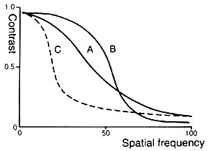
The small graph above shows a very simplistic view of three different optical systems. A: Indicates good resolving power and good contrast. B: Indicates good contrast but poor resolving power. C: Indicates good resolving power but poor contrast.

The MTF graph is the most powerful and detailed way to examine an optical system in detail, and the affects all manner of aberrations have on it. It also allows us to generate accurate simulated images based on the aberrations.

The Test Subject.

The subject i have chosen for the simulated images is the Planet Saturn. Saturn is a good choice as it has features that consist of very high contrast details (its rings and divisions) while its globe consists of very low contrast detail (its belts and zones.)

Part 1. Performance of different aperture sizes.

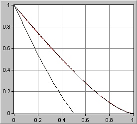
Illustrated here you'll find simulated Planetary images and graphs for 10, 15, 20, 25, 30 and 40cm telescopes. These examples are performed on Saturn at 46" apparent diameter across the major axis of the rings which is typical close to opposition.

Figure 1: An MTF chart generated for two telescopes, one half of the aperture of the other. It is clear how the larger aperture is able to resolve much finer details than the smaller one.

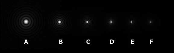
Figure 2: Six different views of the airy disk produced by six different apertures sizes of identical quality with no obstruction or atmospheric turbulence. Its very apparent here why larger telescopes show much finer detail than smaller ones. A: 10cm. B: 15cm. C: 20cm. D: 25cm E: 30cm F: 40cm.

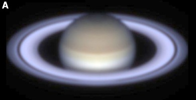
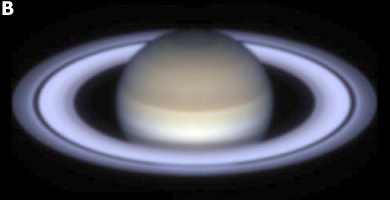
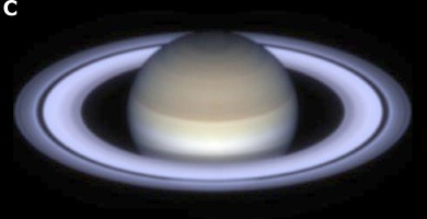
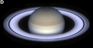
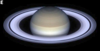
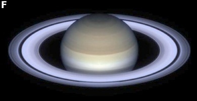
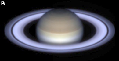
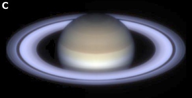
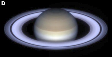
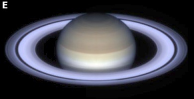
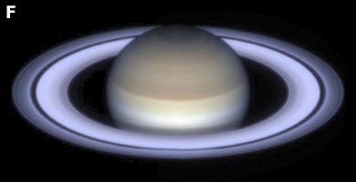
Figure 3: Six different views of Saturn.

A: 10cm aperture. 1/8th wave Spherical Aberration. Unobstructed. No atmospheric turbulence.

B: 15cm aperture. 1/8th wave Spherical Aberration. Unobstructed. No atmospheric turbulence.

C: 20cm aperture. 1/8th wave Spherical Aberration. Unobstructed. No atmospheric turbulence.

D: 25cm aperture. 1/8th wave Spherical Aberration. Unobstructed. No atmospheric turbulence.

E: 30cm aperture. 1/8th wave Spherical Aberration. Unobstructed. No atmospheric turbulence.

F: 40cm aperture. 1/8th wave Spherical Aberration. Unobstructed. No atmospheric turbulence.

Part 2. Performance effects of different size central obstructions.

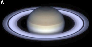
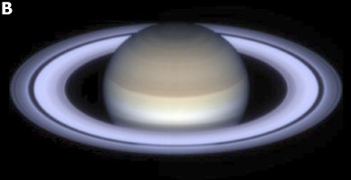
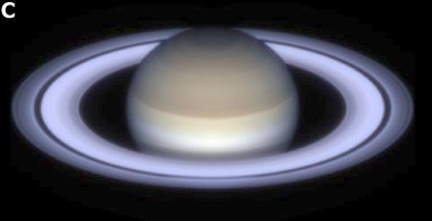
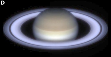
Here we examine Saturn images through a 25cm aperture telescope, with 1/8th wave Spherical Aberration, and no turbulence and a central obstruction size of 0%, 20%, 30% and 50% of the aperture diameter.

Figure 4: Four different views of Saturn.

A: 25cm aperture. 1/8th wave Spherical Aberration. Unobstructed. No atmospheric turbulence.

B: 25cm aperture. 1/8th wave Spherical Aberration. 20% obstruction. No atmospheric turbulence.

C: 25cm aperture. 1/8th wave Spherical Aberration. 30% obstruction. No atmospheric turbulence.

D: 25cm aperture. 1/8th wave Spherical Aberration. 50% obstruction. No atmospheric turbulence.

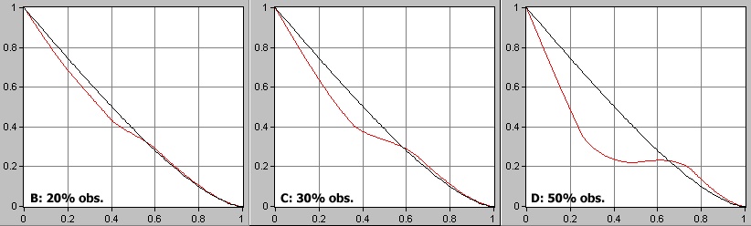
Figure 5: Three MTF graphs showing how the larger the obstruction becomes, the more degraded the performance becomes in the mid to low frequencies (such as Jovian cloud details.) At the high contrast fine detail end (such as Saturn's ring divisions), the performance of the obstructed telescope is slightly superior to an unobstructed aperture. Obstructions larger than about 35% degrade to the mid and low frequency detail to a level not acceptable in Planetary imaging.

We also learn from further examination of the MTF graphs (graphs not published here) that for example a telescope of 25cm aperture with 30% central obstruction will give the same performance on mid-low frequency details (Saturn's belts/zones for example) as an unobstructed instrument with a diameter around 30% less (178mm for a 254mm.) The performance in high frequency details (such as Saturn's rings/divisions) is slightly better for the obstructed instrument than an unobstructed instrument of the same aperture.

Part 3. Performance effects with varying degrees of Spherical Aberration.

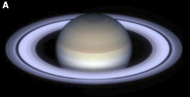
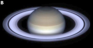
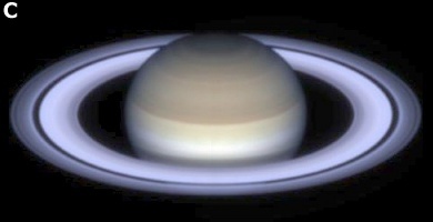
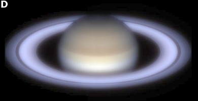
Here we examine the effects of varying degrees of the common optical problem of spherical aberration on Saturn images through an unobstructed 25cm telescope under perfect seeing.

Figure 6: Four different views of Saturn.

A: 25cm aperture. 1/10th wave Spherical Aberration. Unobstructed. No atmospheric turbulence.

B: 25cm aperture. 1/8th wave Spherical Aberration. Unobstructed. No atmospheric turbulence.

C: 25cm aperture. 1/4th wave Spherical Aberration. Unobstructed. No atmospheric turbulence.

D: 25cm aperture. 1/2th wave Spherical Aberration. Unobstructed. No atmospheric turbulence.

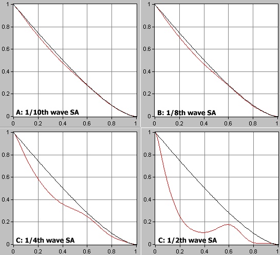
Figure 7: Four MTF graphs showing how varying degrees of spherical aberration affect an unobstructed 25cm telescope under perfect seeing conditions. 1/10th and 1/8th wave levels hardly differ from a perfect aperture. 1/4th wave gives a very similar performance to having a 35% central obstruction. At 1/2 wave all frequencies are seriously degraded and this is an unacceptable level of performance.

Part 4. Performance effects with varying degrees of Atmospheric Turbulence.

Perhaps the most deleterious effect on any optical system is that caused by the ever present Atmospheric turbulence. Below is presented the effects of varying degrees of turbulence on a 25cm, 30% obstructed, 1/8th wavefront system. Images showing the intra and extra focul star images 5 waves defocused, and in focus images are also present in the simulated imagery below.

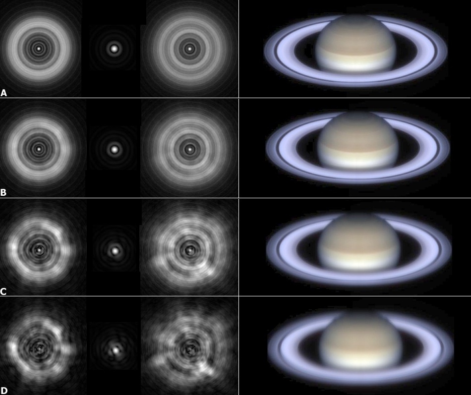
A: 25cm aperture. 1/8th wave Spherical Aberration. 30% obstructed. No atmospheric turbulence.

B: 25cm aperture. 1/8th wave Spherical Aberration. 30% obstructed. 0.05waves RMS atmospheric turbulence.

C: 25cm aperture. 1/8th wave Spherical Aberration. 30% obstructed. 0.15waves RMS atmospheric turbulence.

D: 25cm aperture. 1/8th wave Spherical Aberration. 30% obstructed. 0.25 waves RMS atmospheric turbulence.

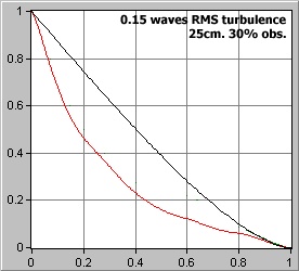
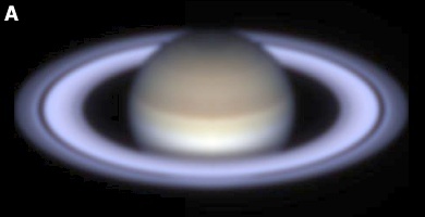
Figure 8: Left: An MTF graph showing the above telescope affected by typical 0.15 waves RMS of turbulence (point C in the above chart) which would be considered a fair rating on the Pickering seeing scale. It becomes very clear how significantly the atmosphere affects what we can hope to record, far more than any of the previous issues since it is something to a very large degree we can not control (unlike quality issues, or collimation etc.) The Graph shows significantly reduced performance across all frequencies. Right: A simulated animation showing a star on a night of fair seeing conditions.

Part 5. Performance effects with different apertures/obstructions/optical errors.

In this section we examine the performance of different size apertures against each other with varying degrees of optical quality and obstruction.

A: 10cm aperture. 1/10th wave Spherical Aberration. un obstructed. No atmospheric turbulence.

B: 15cm aperture. 1/10th wave Spherical Aberration. un obstructed. No atmospheric turbulence.

C: 20cm aperture. 1/4th wave Spherical Aberration. 35% obstructed. No atmospheric turbulence.

D: 25cm aperture. 1/10th wave Spherical Aberration. 30% obstructed. No atmospheric turbulence.

E: 25cm aperture. 1/10th wave Spherical Aberration. 15% obstructed. No atmospheric turbulence.

F: 35cm aperture. 1/4th wave Spherical Aberration. 35% obstructed. No atmospheric turbulence.

From the above simulations we can see how different apertures sizes, with different obstructions and optical quality perform on the same target. Its quite obvious the best performance of all is found in D, E and F images. Of course, these simulations are for perfect seeing conditions - something very rarely seen in larger telescopes from the Earth's surface. For example the simulated 35cm telescope in image E would be far more affected by the atmospheric seeing than the 10 and 15cm apertures in A and B hence those smaller apertures being able to give diffraction limited views a much higher percentage of the time than much larger apertures.

Some final thoughts...

From the information generated, one primary issue of all becomes clear. While smaller high quality apertures, a good amount of the time can give a performance that is very close to the instrument theoretical limit, larger apertures can not due to the limitations imparted by astronomical seeing. But also we have other issues to consider for a telescope best suited to Planetary observation:

1. How big a budget we have.

2. Is the instrument to be permanently located or set-up/transported each time?.

3. How good is the location from which we observe with regard to astronomical seeing?.

Other issues such as collimation accuracy, focus accuracy, thermal equilibrium and above all astronomical seeing are really of much greater concern than the small performance differences that actually exist between telescopes under "lab test" conditions. Also it becomes clear that central obstruction is a greatly overblown issue when its affects are placed against those caused by so many other factors (such as those outlined.)

Perhaps the biggest concern above them all, is user the friendliness of the instrument. After all, we aren't likely to observe very frequently with something that is difficult or frustrating to use. In the end, the best telescope to own is ultimately a trade off of many different issues and its important not to become fixated on a single issue that in the wider perspective of things isn't of great importance.